Many liquidation models use a top-down approach to calculate outcomes for all stakeholders. In Part A and Part B of this series, we reviewed two top-down style liquidation models. They can work very well. But in some situations when many ‘if this, then that’ mechanics come into play and overlap – maybe with convertible notes or when participating preferred calculations are needed – it can be better to use a bottoms-up method. So now in Part C we will review this bottoms-up approach.
The liquidation model itself, for discussion: (available in Downloads → File: Liq_Model_PartC_v1.xlsx). To refresh yourself on the fundraising synopsis, please revisit Part A.
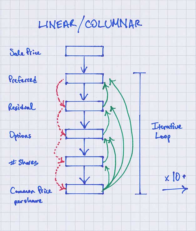
Conceptual Difference: At a high-level the main difference between the top-down and bottom-up methods is the starting point of the logic flow. In a top-down approach we start the calculations with sale price, working down through the liquidation preferences of the preferred shares, calculating down to a price per share for common stock, and dividing up the residual with some iterative calculations. This requires that we define all of the complicated logic and let the model do the per share calculations for us at one or many given sale prices.
In a bottoms-up approach we use our human mind to hard-code (to a degree) the breakpoints – breakpoints being distinct points on the valuation spectrum where an event or clause attached to any security in the waterfall causes a change in the value of any other security. As we do this we also order them from smallest to largest by sale price. Beneficially, we can do the “hard-coding” in either chunks of equity proceeds or on a per common share basis.
That sounds complicated. But it’s harder to explain than to execute. For example, look at the figure below (Figure A).

Figure A – Example breakpoints
We have defined a breakpoint(#4) at an equity proceeds value of $75M, where Series B gets its full liquidation preference, but Series A gets nothing. And then at an equity proceeds level of $80M (breakpoint #5), Series A gets its full liquidation preference, but Common gets nothing yet. Later on, we switched to hard-coding by value per common share, so at $6 (breakpoint #8) both tranches of common options with strike prices of <$6 (tranche Z and Y) would be exercising and receive $2 and $4 per share respectively.
Because we are starting the logic flow by fixing the equity proceeds on a per share basis, the decisions of each stakeholder are easy to figure out.
Almost clear?
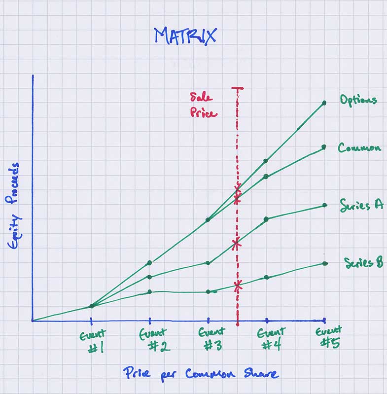
Modeling Methodology Difference: I think it’s helpful to visualize the differences between these modeling styles to make this clearer. Figure B is a picture of how a top-down style model works. Compare this to a visual representation of how a bottoms-up style model functions in Figure C.

Figure B – Top-down visual

Figure C – Bottom-up visual
So the top-down model is essentially linear or columnar and includes all of the logic necessary to calculate per share values for all scenarios (all sale prices) in every column. In the bottoms-up model, we define the breakpoints, laying out the X,Y coordinates in sort of a virtual scatter plot, with as many points needed as there are slope changes in each line. This is the calculation step. And then once the matrix is layed out, we use linear interpolation (what is linear interpolation?) between all of these defined breakpoints to make sure we can calculate all of the per share values of each security at any given sale price.
So in addition to changing the logic flow to work from bottom to top vs top to bottom, we have added an extra spatial dimension to the calculation portion of the model, which makes the logic (all of the if this, then that) easier to lay out. The complexity of Excel formulas involved in the calculations is vastly reduced.
Displaying Results vs Calculating Results: An additional feature of this style of model is that the calculation layer and the display layer are separate – the calculation being the X,Y coordinate matrix and the display being the linear interpolation built on top of that. So depending on the audience you’re presenting the results to (may it be founders, VCs, or a board of directors), you can show whatever exact sale prices are required or beneficial for human digestion, without being constrained by what you need for calculation purposes.
The Catch: Compared to the top-down approach, we have solved a few problems with this style of model. There are no circular references, no iterative calculations needed, and formulas are less complex. But there’s usually a catch. With this approach the model is a little bit harder to rapidly change or build scenarios on. The person laying out the X,Y coordinates of the breakpoints has to take more care in setting and/or resetting them. Mistakes can also be slightly harder to see. But nevertheless this is a very useful tool to improve the “correctness” of a liquidation model when looking at later stage ventures or when a very exact picture of liquidation is required and the details are available to work with.
Please let us know in the comments section if you found this helpful or what other approaches you’ve taken.


